Theory
Theoretical background
Satisfiability Modulo Theories
Satisfiability Modulo Theories (SMT) [1] is concerned with determining the satisfiability of formulas containing both propositional and theory atoms. In this sense, it is a strict generalization of propositional satisfiability (SAT) to formulas that not only contain Boolean variables (as known as propositions), i.e. variables that evaluates to true (\(\top\)) or false (\(\bot\)).
As in SAT, \(SMT(\Delta)\) is a binary decision problem: the formula \(\Delta\) is either satisfiable or unsatisfiable.
\(\Delta\) is sat if there exists a satisfying truth assignment (TA) to the formula’s atoms.
A TA is a mapping:
\[\mu: \text{Atoms}(\Delta) \rightarrow \{ \top, \bot\}\]A TA propositionally satisfies \(\Delta\) if the formula obtained by substituting the atoms with their respective truth values evaluates to \(\top\).
In contrast with SAT, in SMT a TA can be theory unsatisfiable.
A satisfying TA in SMT both propositionally satisfies \(\Delta\) and is theory-satisfiable (denoted \(\mu \models \Delta\) ).
The existence of a satisfying TA implies that there exist at least a value assignment to the variables of the formula that satisfy it. An assignment to the variables of a formula is called a model.
Warning
In SAT, there is a 1-to-1 correspondence between satisfying TA and models, since propositions (i.e. Boolean variables) are the only kind of atoms in propositional logic. The distinction, however, is important in SMT, where atoms can contain non-Boolean variables.
This library focuses on SMT with the theory of linear algebra over reals (SMT-LRA), which enables joint logical / algebraic reasoning. LRA atoms are linear (in)equalities over real variables:
SMT-LRA formulas combine LRA atoms with propositional variables using the standard logical connectives (\(\land, \lor, \rightarrow, \leftrightarrow, \oplus, ...\)), resulting in a flexible formalism for encoding non-convex sets over hybrid discrete/continuous spaces.
For example:
is a SMT-LRA formula having:
3 real variables in 2 LRA atoms
2 propositional variables / atoms
Warning
For ease of exposition, in the following we restrict to SMT-LRA formulas containing LRA atoms only (i.e. Boolean variables). The extension of the definitions to formulas with propositional variables is straightforward and can be found in the cited papers.
SMT is a centerpiece in automated reasoning and has found many practical applications, in particular in the formal verification of software and hardware systems. More recently, SMT has been applied to the verification of machine learning models.
Example 1
Let \(w_1, ..., w_N\) be the parameters of a rectified linear unit (ReLU) over inputs \(x_1, ... , x_N\). The unit can be encoded with the following SMT-LRA formula:
where \(h\) denotes the pre-activation value of the unit.
SMT solvers are widely used for reasoning on a trained neural network, therefore the parameters \(w_i\) are real constants.
A ReLU unit is said to be firing if it propagates a signal, i.e.:
For a given subset of its inputs, a ReLU unit can be:
inactive if it never fires
active if it always fires
unstable otherwise
Using SMT, it is possible to determine if the unit is inactive given an interval:
The unit is inactive in \(I\) if and only if the following SMT calls
returns unsat, indicating that there doesn’t exist an assignment to \(x_1, ..., x_N\) for which the formula evaluates to true.
Our library builds upon pysmt for defining SMT-LRA formulas.
Code Example 1
The following code implements Example 1 for a toy scenario with 2 input variables. The parameters are set to \(\mathbf{w} = [1,1]\) for simplicity in the following examples.
import pysmt.shortcuts as smt

### the ReLU unit encoding

x1 = smt.Symbol("x1", smt.REAL)  # input variables
x2 = smt.Symbol("x2", smt.REAL)
xvec = [x1, x2]

h = smt.Symbol("h", smt.REAL)  # pre-activation value
y = smt.Symbol("y", smt.REAL)  # post-activation value

w1 = smt.Real(1)  # the unit (constant) parameters
w2 = smt.Real(1)
wvec = [w1, w2]

# h is the linear combination of xvec and wvec
preactivation = smt.Equals(
    h, smt.Plus(*[smt.Times(xvec[i], wvec[i]) for i in range(2)])
)

# y is max(0, h)
postactivation = smt.Ite(
    smt.LE(h, smt.Real(0)), smt.Equals(y, smt.Real(0)), smt.Equals(y, h)
)
# if-then-else: Ite(a, b, c) is shorthand for (a -> b) and (not a -> c)

unit = smt.And(preactivation, postactivation)


### PROBLEM: is the unit inactive given an interval I?

firing = smt.GT(y, smt.Real(0))

# I1: x1, x2 in [-1, 1]
I1 = smt.And(
    smt.LE(smt.Real(-1), x1),
    smt.LE(x1, smt.Real(1)),
    smt.LE(smt.Real(-1), x2),
    smt.LE(x2, smt.Real(1)),
)

# I1: x1, x2 in [-1, 0]
I2 = smt.And(
    smt.LE(smt.Real(-1), x1),
    smt.LE(x1, smt.Real(0)),
    smt.LE(smt.Real(-1), x2),
    smt.LE(x2, smt.Real(0)),
)

print("inactive in I1?", not smt.is_sat(smt.And(unit, firing, I1)))
print("inactive in I2?", not smt.is_sat(smt.And(unit, firing, I2)))

# >>> inactive in I1? False
# >>> inactive in I2? True
Check the pysmt documentation for more examples and an in-depth discussion on SMT.
From qualitative to quantitative reasoning
SMT-LRA enables qualitative algebraic / logical reasoning, for instance, it can be used to decide whether a certain property is satisfied by a neural network or not. What it can’t be used for is quantitative analysis on the satisfaction of a formula (e.g. the probability of satisfaction).
In order to enable quantitative reasoning on top of SMT, a few aspects have to be addressed.
First, instead of searching for a single satisfying TA, we need to enumerate them all, i.e., compute a set \(M\) such that:
\(\forall \mu \in M \:.\: \mu \models \Delta\) (they satisfy the formula)
\(\forall \mu_i, \mu_j \in M \:.\: i \neq j \implies \mu_i \land \mu_j \models \bot\) (they are mutually disjoint)
\(\cup_{\mu \in M} \equiv \Delta\) (they form a complete partitioning of the formula)
Example 2
Consider the ReLU encoding in Example 1. The formula \(Unit\) defines two convex regions of the input space:
Second, we need to be able to quantify the number of models for each satisfying TA. In LRA, models are typically uncountable. We can, however, compute the volume of a satisfying TA:
where \(\int_\mu\) denotes an integral restricted to \(\mu\). \(vol(\mu)\) is finite if \(\mu\) is a closed polytope.
Example 3
Consider the formula
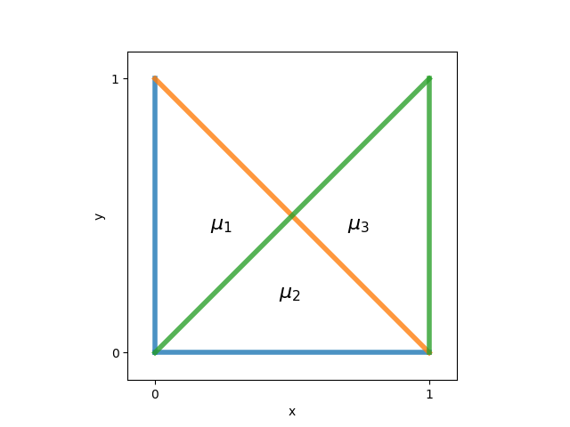
The set of satisfying TAs is (omitting always true atoms \((0 \le x), (0 \le y), (x \le 1)\)):
each having equal volume \(vol(\mu_i) = \int_{\mu_i} 1 \: dx dy = 1/4\).
We can easily generalize the concept of volume from TAs to arbitrary formulas:
\[vol(\Delta) \equiv \sum_{\mu \models \Delta} vol(\mu)\]
This is useful when we want to compute ratios of satisfaction. In Example 3, we can conclude that \(x \ge y\) is satisfied by 2/3 of the models of \(\Delta\).
Notice that, so far, each model has the same “importance” in our quantitative calculations. In probabilistic terms, we would say that models are uniformly distributed.
Weighted Model Integration
Weighted Model Integration (WMI) [2] is a formalism introduced in the context of probabilistic inference with logical and algebraic constraints.
Simply put, quantitative SMT-LRA reasoning is complemented with a notion of weight. A weight is defined by two ingredients:
a weight function \(w\), which associates a non-negative value to models
a weight support \(\chi\), which restricts the domain of \(w\)
The weighted model integral of a weighted SMT-LRA formula \(\langle \chi, w \rangle\) is defined as:
In theory, the only prerequisite for \(w\) (aside from non-negativity) is to be integrable over convex polytopes. In practice, most approaches in WMI consider piecewise polynomial weights. The reason is twofold:
They are arbitrary approximators (Stone-Weierstrass theorem)
They are easy to work with, being closed under the following operations: \(+, \cdot, \int_\mu\)
wmpy uses the pysmt formulas for defining the weight. In
practice, while the support is a standard SMT-LRA formula, the weight
function is an LRA term, i.e. an expression that does not evaluate to
true or false.
Code Example 2
The following code implements the quantitative analysis introduced in Example 3 with two different weight functions:
constant 1 (i.e. unweighted)
the quadratic polynomial \(x^2 + 1\)
# now we import everything in order to avoid the "smt." clutter
from pysmt.shortcuts import *

# wmpy's design is modular
from wmpy.solvers import WMISolver

# in this example, we pair total TA enumeration...
from wmpy.enumeration import TotalEnumerator

# ...with exact integration based on the LattE integrale software
from wmpy.integration import LattEIntegrator


x = Symbol("x", REAL)
y = Symbol("y", REAL)

# the support is the formula from Example 3
support = And(
    LE(Real(0), x),
    LE(Real(0), y),
    Or(
        LE(Plus(x, y), Real(1)),
        And(GE(x, y), LE(x, Real(1))),
    ),
)

# we consider two different weights
weight1 = Real(1)
weight2 = Plus(Pow(x, Real(2)), Real(1))

for w in [weight1, weight2]:

    # solvers are designed to answer multiple queries given a pair <support, w>
    # hence, the pair is passed as a parameter to the enumerator
    enumerator = TotalEnumerator(support, w, get_env())
    integrator = LattEIntegrator()

    wmi_solver = WMISolver(enumerator, integrator)

    # we set query to true in order to compute the full WMI of <support, w>
    query = Bool(True)
    print(f"The WMI of {serialize(w)} is:", wmi_solver.compute(query, {x, y})["wmi"])

# >>> The WMI of 1.0 is: 0.75
# >>> The WMI of ((x ^ 2.0) + 1.0) is: 1.0104166666666667
More complex weight functions can be defined by combining valid weight terms by means of If-Then-Else expressions.
For instance, the following code defines a univariate triangular distribution with domain \([-l, u]\) and mode \(m\):
from pysmt.shortcuts import *

x = Symbol("x", REAL)

height = 2 / (u - l) # ensures a normalized distribution

a1 = height / (m - l)
b1 = -a1 * l

a2 = height / (m - u)
b2 = -a2 * u

support = And(LE(Real(l), x), LE(x, Real(u)))

linear = lambda a, b : Plus(Times(Real(a), x), Real(b))

w = Ite(LE(x, Real(m)), linear(a1, b1), linear(a2, b2))